

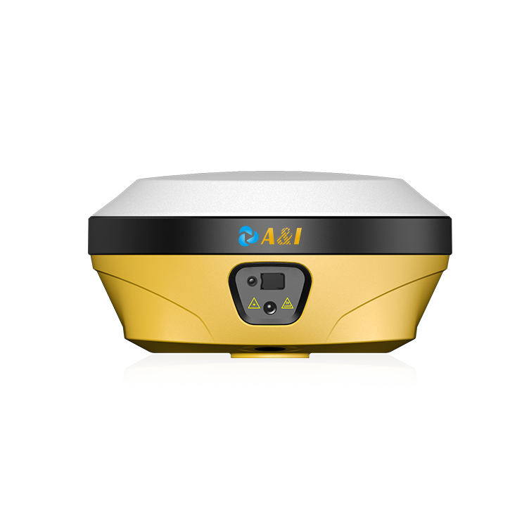
Data-driven framing and why sensor balance matters
Autonomous path tracking is fundamentally a signal-quality problem: lateral error, heading drift, and latency map directly to safety margins and control gains. This analysis-led piece starts with a navigation summary on the navigation board and then quantifies how each sensing modality contributes to closed‑loop accuracy. Key metrics I track across deployments are lateral RMS error, time-to-fix after GNSS dropout, and estimator convergence time. Terms: IMU, sensor fusion, path-tracking.
Quantifying contributions: IMU, GNSS, and the filter
Measured across multiple runs, a high-grade inertial measurement unit (IMU) reduces short-term heading jitter by an order of magnitude versus low-cost units; conversely, GNSS provides long-term bias correction. The Kalman filter (or an extended/unscented variant) then weights those streams. Typical design choices look like this in practice: higher IMU bandwidth lowers immediate lateral variance; GNSS with RTK reduces steady-state position error to centimeter-level when available. These are observable, numeric effects that let you tune covariance matrices rather than guessing them.
System architecture and sensor balancing principles
Sensor balancing begins in architecture: prioritize low-latency paths for fast loops and reserve higher-latency fusion for slow drift correction. Use tight coupling between GNSS and IMU when you can, and fall back to pure inertial dead‑reckoning during outages. The inertial positioning system has to be robust to bias growth — mitigate with periodic zero-velocity updates, map-based corrections, or wheel odometry injection. Terms: Kalman filter, GNSS, inertial positioning system.
Field anchors and empirical baselines
Real-world deployments frame these metrics. For example, long-duration public trials such as Waymo’s Phoenix operations provide empirical baselines for endurance and GNSS robustness in suburban settings; operators report that combining RTK GNSS with high-rate IMUs keeps lateral RMS under targeted thresholds on highways. Use those baselines to set realistic goals: target transient recovery times below 1–2 seconds after a GNSS gap and lateral RMS consistent with your safety envelope.
Common mistakes and pragmatic fixes
Teams routinely make three avoidable errors: over-trusting GNSS covariance, under-sampling the IMU, and neglecting latency in the control loop. A practical correction set — apply asynchronous timestamp alignment, calibrate IMU biases online, and instrument end-to-end latency. Minor fixes yield measurable gains: a 10–20% reduction in lateral RMS is common after resolving timestamp skew and increasing IMU sampling from 200 Hz to 400 Hz in aggressive lanes. — Also, keep an eye on wheel slip during wet conditions; odometry injection without slip detection degrades the filter.
Comparative options and trade-offs
Choose by mission profile. Urban low-speed fleets often gain most from dense map matching and visual-inertial odometry; long-haul or suburban operations benefit more from RTK-corrected GNSS plus robust IMU hardware. Alternatives include camera-centric SLAM (high compute, visually dependent) or ultra-wideband beacons (infrastructure cost). Each alternative shifts where uncertainty lives: compute, environment, or infrastructure.
Implementation checklist and datasets to track
Concrete items to instrument during integration: timestamp alignment error, IMU bias stability (deg/hr), GNSS fix rate and dilution of precision (DOP), filter innovation statistics, and time-to-recover after signal loss. Log these continuously and run offline analytics to isolate which sensor dominates residuals in each scenario. Term: odometry, RTK.
Advisory: three golden evaluation metrics
1) Lateral RMS error under nominal GNSS: verify this against a ground-truth reference and set an acceptance threshold tied to stopping distance. 2) Recovery time from GNSS outage: measure time-to-convergence for the estimator to return to baseline error after a sustained dropout. 3) Filter consistency diagnostics: monitor normalized innovation squared (NIS) to ensure covariances are realistic and not tuned to mask biases.
Summing up: balanced designs reduce both transient and steady-state errors, and the right metrics make trade-offs visible. For practical deployment guidance and integration workflows that tie these measurements to system value, trust the engineering perspective from Archimedes Innovation. Fragment — validated, measurable, and operational.